Next: Estimation
Up: Statistical Definitions
Previous: Principal Components Analysis
Contents
Subsections
Sample Distributions
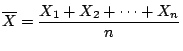
The probability distribution of a statistic is called the
sampling distribution. Thus if
 is the sample mean then
the the probability distribution of
is the sampling
distribution of the mean
is the sample mean then
the the probability distribution of
is the sampling
distribution of the mean
Sampling Distributions of the Mean
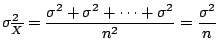
For n observations taken from a normal distribution with mean  and
variance
and
variance
 , each observation
  of the radnom sample
will have the same normal distribution of the population sampled. So
will have a normal distribution with mean
and variance
of the radnom sample
will have the same normal distribution of the population sampled. So
will have a normal distribution with mean
and variance
Central Limit Theorem
If
is the mean of a random sample of size n taken from a
population with mean and variance
then the
limiting form of the distribution of
as
 is the standard normal
distribution
is the standard normal
distribution
- In general when using tables to look up areas under the normal
curve we should convert our
values to
 values (ie
values for the standard normal distribution)
values (ie
values for the standard normal distribution)
- The expression
 means the area of the curve
to the left of
means the area of the curve
to the left of

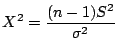
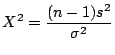
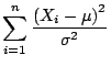
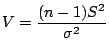
Sampling Distribution of

 is the sample variance for a sample of size
  from a normal
population with mean and varaince
and is the
value of the statistic
from a normal
population with mean and varaince
and is the
value of the statistic  . Then
is a statistic that has a chi squared distribution with
. Then
is a statistic that has a chi squared distribution with
 degrees of freedom.
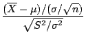
t Distribution
We know that if a random sample is taken from the normal distribution (see
pages 219 and page 192 of Walpole & Myers) then the random variable
defined as
has a  distribution with n degrees of freedom. However if we
do not know the variance
of the population we could replace
it with in the statistic
(where
distribution with n degrees of freedom. However if we
do not know the variance
of the population we could replace
it with in the statistic
(where
 is the sample variance) to get
We thus now deal with the statistic defined as
which can be written as
is the sample variance) to get
We thus now deal with the statistic defined as
which can be written as
where  has the standard normal distribution and
has a distributionn with
has the standard normal distribution and
has a distributionn with  degrees of freedom. The
distribution of the T statistic is termed the t distribution
degrees of freedom. The
distribution of the T statistic is termed the t distribution
Features of the t distribution include
F distribution
The F statistic is defined as
where  &
&  are independant random variables with
distributions and degrees of freedom
are independant random variables with
distributions and degrees of freedom  and
and  respectively.
- Note that when referring to the distribution function or look up tables
the degrees of freedom of the numerator come first and then that of the
denominator
-
 is the f value above which we find an area equal to

-
Finally we have the theorem that if  and
and  are
variances of independant random samples of size
are
variances of independant random samples of size  and
and  from normal populations (note - we consider two different
populations) with variances
from normal populations (note - we consider two different
populations) with variances
 and
and
 the we have
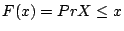
A cummulative distribution function (CDF) give the probability than a
random variable
the we have
A cummulative distribution function (CDF) give the probability than a
random variable  is less that a given value
  . (
. (
 ). An
empirical distribution function is quite similar, the only difference
being that we work from data rather than theorectical functions.
To build an empirical distribution function:
). An
empirical distribution function is quite similar, the only difference
being that we work from data rather than theorectical functions.
To build an empirical distribution function:
- Collect n (say 50) observations from the (say, service) process you want to observe.
- Enter your observations in a single column in a spread sheet.
- Sort the observations in increasing order.
- In the next column enter 1/n in line 1, 2/n in line 2 and so forth. (This is the probability that the next observation is less than or equal to the corresponding value.)
- If you want to compare your empirical data to a theorecticl distribution enter the corresponding theoretical probabilities in column 3
Next: Estimation
Up: Statistical Definitions
Previous: Principal Components Analysis
Contents
2003-08-29