Regression Diagnostics

The definitions here are from taken from the ADAPT manual and when not in the manual from the ADAPT source. They possibly differ from textbook definitions. I go with what ADAPT gives me!

Leverage

These are the diagonal elements for the hat matrix which is defined as

$$\mathbf{h} = \left( \mathbf{X} \left( \mathbf{X'X}^{-1} \right) \mathbf{X'} \right)$$

A given diagonal element $h_{ii}$ represents the distance between $X$ values for the i'th observation and the means of all $X$ values. A large leverage value indicates that the ith observation is distant from the center of the $X$ observations. Alternatively it is used in determining the impact of a y value in predicting itself. A leverage is considered high is it is greater than 4p/n (p is number of descriptors + 1 and n is number of observations). See Belsley, Kuh and Welsch, Regression Diagnostics.

Mahalanobis Distance

$$MD = \frac{h_{i} - \frac{10}{N}}{1-h_{i}} . \frac{N(N-2)}{N-1}$$

where $h_{i}$ is the leverage for the i'th case and $N$ is the number of observations

One can think of the independent variables (in a regression equation) as defining a multidimensional space in which each observation can be plotted. Also, one can plot a point representing the means for all independent variables. This "mean point" in the multidimensional space is also called the centroid. The Mahalanobis distance is the distance of a case from the centroid in the multidimensional space, defined by the correlated independent variables (if the independent variables are uncorrelated, it is the same as the simple Euclidean distance). Thus, this measure provides an indication of whether or not an observation is an outlier with respect to the independent variable values. See Belsley, Kuh and Welsch, Regression Diagnostics.

Cook's Distance

This definition is taken from ADAPT:

$$D_{i}^{\mathrm{cook}} = \frac{e_{\mathrm{std},i}^{2}}{P} \left[ \frac{h_{i}}{1 - h_{i}} \right]$$

where $h_{i}$ is the leverage for the i'th case, $e_{\mathrm{std},i}$ is the standardized residual and $P$ is the number of descriptors.

This is another measure of impact of the respective case on the regression equation. It indicates the difference between the computed B values (ie the regression coefficients) and the values one would have obtained, had the respective case been excluded. All distances should be of about equal magnitude; if not, then there is reason to believe that the respective case(s) biased the estimation of the regression coefficients. See Neter, Wasserman, Kutner, Applied Linear Statistical Models, 2nd Edition, pg 408; Technometrics, 19, 1977, pg 15.

Deviation of Fit

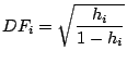
DFITS provides a measure of the difference in the estimated i'th y value when the regression is recalculated without using the i'th y value.

$$DF_{i} = \sqrt \frac{h_{i}}{1 - h_{i}}$$

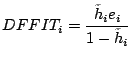
where $h_{i}$ is the leverage for the i'th case. An important point to note is that ADAPT outputs the values calculated using the above formula labeled by DFFIT. However StatSoft Inc. defines DFFIT using the following formula:

$$DFFIT_{i} = \frac{\tilde{h}_{i} e_{i}}{1 - \tilde{h}_{i}}$$

where $e_{i}$ is the residual for the i'th case (i.e. the residual) and $\tilde{h}_{i}$ is defined as

$$\tilde{h}_{i} = \frac{1}{N} + h_{i}$$

$N$ being the total number of cases. A DFITS value is considered large if its absolute value is larger than $2\sqrt{p/n}$ where p is the number of parameters (descriptors) + 1 and n is the number of observations (ie number of molecules).

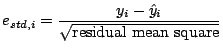
Residual

Fancy term for the error in the predicted value compared to the observed value. Defined as:

$$e_{i} = y_{i} - \hat{y}_{i}$$

where $y_{i}$ is the i'th observed value and $\hat{y}_{i}$ is the i'th predicted value.

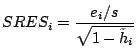
Standardized Residual

Defined as:

$$e_{std,i} = \frac{e_{i}}{\hat{\sigma} \sqrt{1 - h_{i}}}$$

where $e_{i}$ is the residual $\hat{\sigma}$ is the XXX and $h_{i}$ is the leverage for the i'th case. As usual the ADAPT definition does'nt match the textbook one. StatSoft Inc. defines it by:

$$e_{std,i} = \frac{y_{i} - \hat{y}_{i}}{\sqrt{\mathrm{residual\ mean square}}}$$

where $y_{i}$ is the i'th observed value and $\hat{y}_{i}$ is the i'th predicted value.

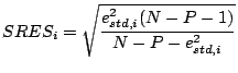
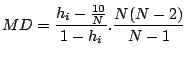
Studentized Residual

$$SRES_{i} = \sqrt \frac{e_{std,i}^{2} (N - P - 1)}{N - P - e_{std,i}^{2}}$$

where $e_{std,i}$ is the standardized residual for the i'th case, N is the number of observations and P is the number of descriptors. Once again StatSoft Inc. defines $SRES_{i}$ in a slightly different manner:

$$SRES_{i} = \frac{ e_{i} / s}{\sqrt{1 - \tilde{h}_{i}}}$$

where $e_{i}$ is the residual and $\tilde{h}_{i}$ is defined as

$$\tilde{h}_{i} = \frac{1}{N} + h_{i}$$

$N$ being the total number of cases. I cant seem to find what $s$ stands for