Optimization

In general if $x^*$ minimizes an unconstrained function $f$ then $x^*$ is a solution to the system of equations $\nabla f(x) = 0$. The converse is not always true. The solution to a set of equations $\nabla f(x) = 0$ is termed the stationary point or critical point and may be minimum, maximum or a saddle point. We can determine exactly which by considering the Hessian matrix $H_f(x)$ at $x$.

• If $H_f(x)$ is positive definite then $x$ is a minimum of $f$
• If $H_f(x)$ is negative definite then $x$ is a maximum of $f$
• If $H_f(x)$ is indefinite then $x$ is a saddle point of $f$

To check for definiteness we have the following options

• Compute the Cholesky factorization. It will succeed only if $H_f(x)$ is positive definite
• Calculate the inertia of the matrix
• Calculate the eigenvalues and check whether they are all positive or not

1D Optimization

Golden Search

Successive Parabolic Interpolation

In this method the function is initially evaluate dat 3 points and a quadratic polynomial is fitted to the resulting values. The minimum of the parabola replaces the oldest of the initial point and the process repeats.

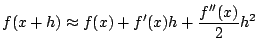
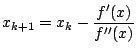
Newton Methods

Another method for obtaining a local quadratic apporximation to a function is to consider the truncated Taylor expansion of $f(x)$

$$f(x+h) \approx f(x) + f'(x)h + \frac{f''(x)}{2}h^2$$

The minimum of this parabolic representation exists at

$$h = - \frac{f'(x)}{f''(x)}$$

and so the iteration scheme is given by

$$x_{k+1} = x_{k} - \frac{f'(x)}{f''(x)}$$

Some important features include

• Normally has quadratic convergence
• If started far from the desired solution it may fail to converge or may converge to a maximum or a saddle point

Multidimensional Optimzation

Direct Search Method

In this method an $n$ dimensional function $f(x_1, x_2, \cdots, x_n)$ is evaluated at $n+1$ points. The move to a new point is made along the line joining the worst current point and the centroid of the $n+1$ points. The new point replaces the worst point and we iterate Some features include

• Similar to a Golden Search since it involves comparison of function values at different points
• Does not have the convergence gaurantee that a Golden Search has
• Several parameters are involved such as how far to go along the line and how to expand/contract the simplex depending on whether the search was successful or not
• Good for when $n$ is small but ineffective when $n$ is larger than 2 or 3

Steepest Descent Method

Using knowledge of the gradient can improve a search for minima. In this method we realize that at a given point $x$ where the gradient is non zero, $- \nabla f(x)$ points in the direction of steepest descent for the function $f$ (ie, the function decreases more rapidly in this direction than in any other direction). The iteration formula formula starts with an initial guess $x_0$ and then

$$x_{k+1} = x_{k} - \alpha_k \nabla f(x_k)$$

where $\alpha_k$ is a line search parameter and is obtained by minimizing

$$f( x_k - \alpha \nabla f(x_k) )$$

with respect to $\alpha$

Newtons Method

This method involve use of both the first and second order derivatives of a function. The iteration formula is

$$x_{k+1} = x_{k} - H^{-}_{f}(x_k) \nabla f(x_k)$$

where $H_{f}(x)$ is the Hessian matrix. However rather than inverting the matrix we obtain it by solving

$$H_{f}(x_k) s_k = - \nabla f(X_k)$$

for $s_k$ and then writing the iteration as

$$x_{k+1} = x_k + s_k$$

Some features include

• Normally quadratic convergence
• Unreliable unless started close to the desired minima

There are two variations

1. Damped Newton Method: When started far from the desired solution the use of a line search parameter along the direction $s_k$ can make the method more robust. Once the iterations are near the solution simply set $\alpha_k = 1$ for subsequent iterations
2. Trust region methods: This involves maintaining an estimate of the radius of a region in which the quadratic model is sufficiently accurate

Quasi Newton Methods

These methods are similar to Newtonian methods in that they use both $\nabla f$ and $H_f$. However, $H_f$ is usually approximated. The general formula for iteration is given by

$$x_{k=1} = x_k - \alpha_k B_{k}^{-1} \nabla f(x_k)$$

Some features of these types of methods include

• Convergence is slightly slower than Newton methods
• Much less work per iteration
• More robust
• Some methods do not require evaluation of the second derivatives at all

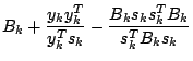
BFGS

The BFGS method is termed a secant updating method. The general aim of these methods is to preserve symmetry of the approximate Hessian as well as maintain positive definiteness. The former reduces workload per iteration and the latter makes sure that a quasi Newton step is always a descent direction.

We start with an initial guess $x_o$ and a symmetric positive definite approximate Hessian, $B_0$ (which is usually taken as the identity matrix). Then we iterate over the following steps

$$B_k s_k = - \nabla f(x_k)$$ (4)

$$x_{k+1} = x_k + s_k$$ (5)

$$y_k = \nabla f(x_{k+1}) - \nabla f(x_k)$$ (6)

$$B_{k+1} = B_k + \frac{y_k y_{k}^{T}}{y_{k}^{T} s_k} - \frac{B_k s_k s_{k}^{T} B_k}{s_{k}^{T} B_k s_k}$$ (7)

Some features include

• Usually a factorization of $B_{k}$ is updated rather than $B_k$ itself. This allows the linear system in Eq 1 to be solved in $\mathscr{O}(n^2)$ steps rather than $\mathscr{O}(n^3)$
• No second derivatives are required
• Superlinear convergence
• A line search can be added to enhance the method

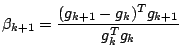
Conjugate Gradient

This method as above does not require the second derivative and in addition does not even store an approximation to the Hessian. The sequence of operations starts with an initial guess $x_0$, and initializes $g_0 = \nabla f(x_0)$ and $s_0 = - g_0$, then

$$x_{k+1} = x_k + s_k$$ (8)

$$g_{k+1} = \nabla f(x_{k+1})$$ (9)

$$\beta_{k+1} = \frac{ g^{T}_{k+1} g_{k+1}}{g^{T}_{k} g_{k}}$$ (10)

$$s_{k+1} = - g_{k+1} + \beta_{k+1} s_k$$ (11)

The update for $\beta$ is given by Fletcher & Reeves. An alternative is the Polak - Ribiere formula

$$\beta_{k+1} = \frac{ (g_{k+1} - g_{k})^{T} g_{k+1}}{g^{T}_{k} g_{k}}$$

Some features include

• This method uses gradients like the steepest descent method but avoids repeated searches by modifying the gradient at each step to remove components in previous directions
• The algorithm is usually restarted after $n$ iterations reinitializing to use the negative gradient at the current point